convergence & variance

I've been self-studying and reviewing some old results in classical statistics & probability theory to help gain better intuitions regarding probability statements at work. Two concepts that I think are worth understanding in more detail are convergence & variance.

Convergence

Convergence in calculus is fairly straightforward; as n-> infinity, we can make some statements as to what the value of some continuous function trends to or tends towards as a result of that. Why does this require more nuance in probability?

Suppose we have the analagous situation where we have X1..Xn all drawn from N(0,1) distribution. We would then probably want to say that as n-> infinity, Xn -> N(0,1). However, two continuous distributions can never "equal" each other. As in P(Xn=N(0,1)) = 0.

Another example that demonstrates this difficulty is looking at the distribution X_n ~ N(0, 1/n). As n-> infinity, then the variance of the distribution is going down. Then we would like to say Xn -> 0. However, P(Xn = 0) = 0, since for any continuous distribution, the probability that equals a single value is 0. Again, seems like semantics, but I suppose some mathematicians have tried for a bit more of a rigorous approach.

To get around this, we make the following two statments of probability:

1. We say Xn -> X (in probability) when, for some positive epsilon e, P(|xn-x| > e) -> 0.
2. We say Xn -> X (in distribution) when, limit as n-> inifinity Fn(t) -> F(t), where F(t) is the CDF of X evaluated at t.

Key Results in Probabilty Theory We all throw around the terms "Law of Large Numbers" and Central Limit Theorem. Here is a quick summary and overview of what those terms actually mean. the Weak LLN states that:

Let X1...Xn be iid with mean u and variance s^2. Let X_bar_n be the sample mean. Then as n-> infinity X_bar_n converges in probability to u.

So what does this tell us? As we take more and more samples, we know that the sample mean will start to cluster closer and closer to u.

While useful, this does not allow us to make probability statements about the sample mean. For example, we might want to make statements about the uncertainty in our estimation, such as a confidence bound. For that, we would need to make a claim about the distribution of our sample mean (which is different from the distribution that Xi is actually drawn from).

The Central Limit Theorem states that:

Let X1...Xn be iid with mean u and variance s^2.  Let X_bar_n be the sample mean. Then X_bar_n converges in distribution to N(u, s^2/n). 

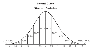
This allows us to make a probability statement about X_bar_n. Note that the CLT can come in many different forms, all of which are the same. For example, another common form that we see is that sqrt(n) * (X_bar_n - u) / s --> N(0, 1). This is the same, as what is written above. If we subtract the mean from a distribution , then we shift it down to have a mean of 0. If the variance of the original distribution is s^2/n, it is a property of variance that Var(a * X) = a^2 * Var(X). From this fact it becomes obvious to see how we can reverse engineer the other forms of the CLT. (we want to cancel out and get a variance of 1)

Variance & Bets

We can also make other useful statements about X_bar_n. Let X1...Xn be also drawn iid from some distribution with finite mean and variance u, s^2. Var(x1) = s^2, E(x1) = u. Then X_bar_n is the average of a "n" samples. If the variance of each individual sample is s^2, and they are idependently distributed, then we can use the property that Var(x+y) = Var(x) + Var(y) if x & y are independent. Combine this with the property that the 1/n part of taking the sample mean is a constant, we have that Var(X_bar_n) = (n * s^2) / n^2 == s^2 /n, which is what we saw before in CLT!

Putting it all together:

1. We know that as we increase the samples, our sample mean starts to get clustered around the actual mean of the distribution we are drawing from
2. The distribution of our sample mean will be normally distributed around that mean, with its variance decreasing as n increases.

This is useful because variance is important when making bets. A good mental model for any hedge-fund or bettor is the following: Sharpe = Edge * sqrt(n_bets). Sharpe is the ratio of returns to volatility (which is just standard deviation). Edge can be treated as the extra return you have over the average player. With the above information in hand, we can infer where all of this is coming from. Imagine we make n-bets, all with the same expected value u, and variance s^2. If we make a single bet, (i.e our n ==1), then volatiliy = sqrt(n), by defn.

however, if we average our returns (basically take X_bar_n), then the result we just learned is that our expected return will be the same, but our variance scales by s^2/n. Therefore, our sharpe ratio goes up by a factor of root(n)! Which explains the need to diversify the markets and bets you are making.